Optimizing Heat Transfer: Dissolved Gas in Cooling-Tower Working Fluid

Why we ran this

Water is the working fluid of choice for large-scale cooling because its specific heat is high: a given mass of it carries away more heat than almost anything else you could pump. In Southern Nevada, where this work was done, that virtue collides with a constraint. Lake Mead has dropped roughly a hundred and seventy feet, the federal government has issued a tier-two shortage declaration, and evaporative cooling towers on commercial buildings are one of the larger discretionary draws on the remaining supply.

The obvious lever is to make each litre carry more heat. If it does, the tower can hold the same load at a lower circulation rate and evaporate less. So we asked a narrow, testable question:

Does water carrying dissolved gas remove more heat than the same water without it?

This post is the bench work that answers it, published as it was written up in May 2023 — hardware, method, energy balance, the raw curves and the parts that did not come out the way we expected.

The treatment hardware

Water was treated with a CTR-PACK — the cooling-tower retrofit build of our recirculating gas-injection module. It draws 2.8 kW continuously, moves 40 GPM, and carries an oxygen concentrator, an ozone generator and an auxiliary port for injecting outside gas, which is what let us run the same experiment on oxygen and on plain atmospheric air without changing anything else.

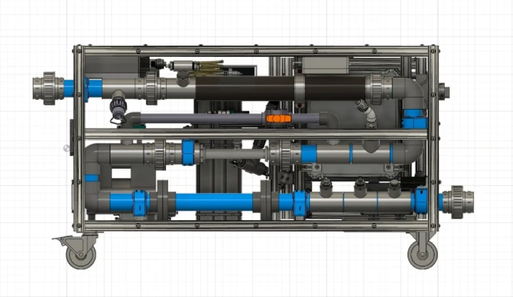
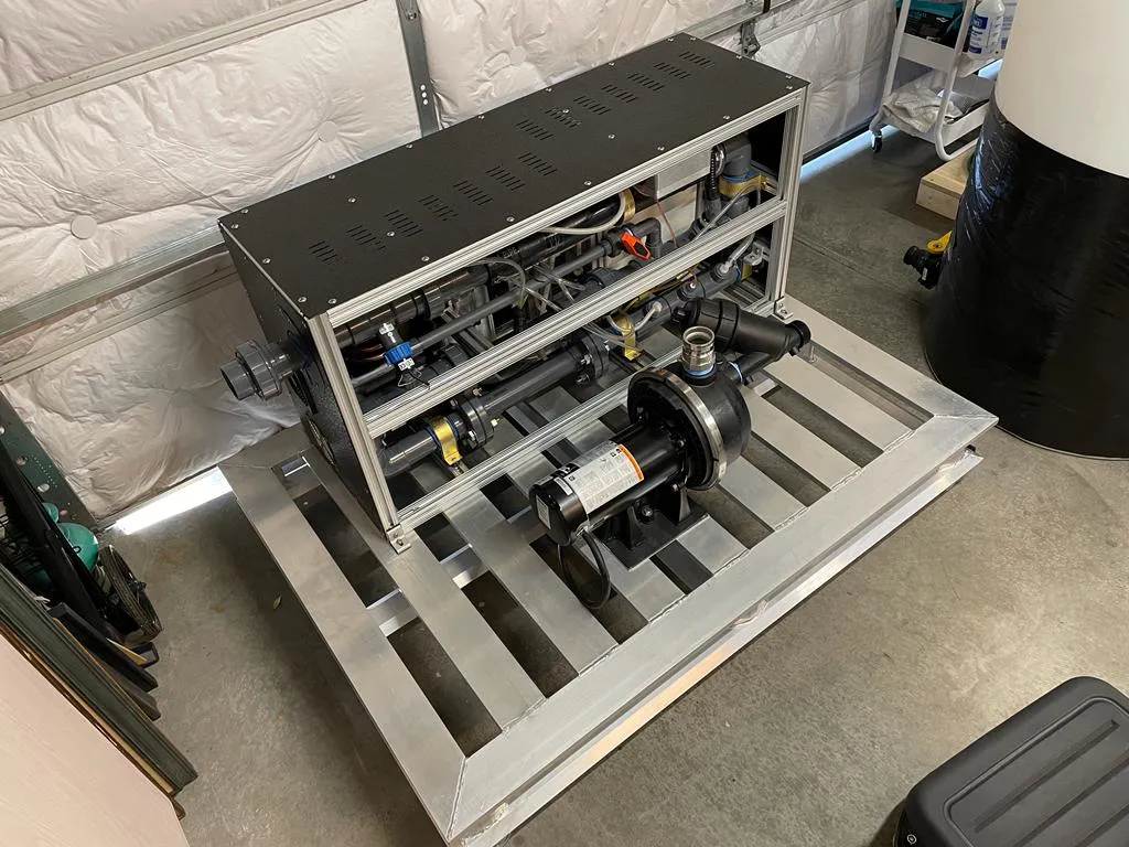
That last point matters for reading the cost figures at the end. The 2.8 kW draw is the draw of a machine built to do many jobs. A unit built to do only this one would draw less, and the energy comparison below is therefore pessimistic about the treatment, not generous to it.

The bench

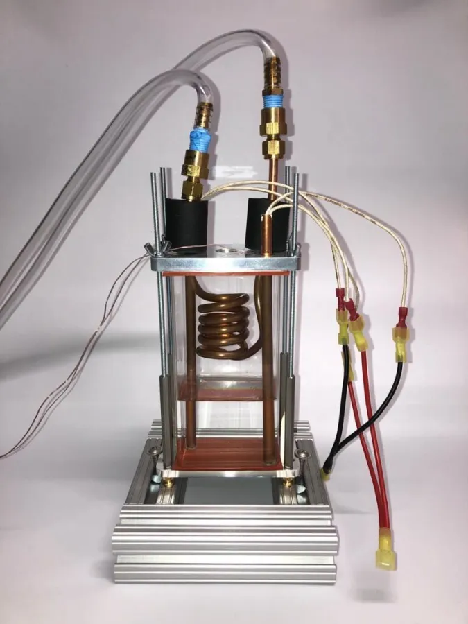
The test chamber is a rectangular glass tube clamped between two aluminium plates. Two cartridge heaters sit inside copper tubes sealed with copper foil and boil the fluid in the chamber; a copper coil above them condenses the vapour. The coil is fed by a recirculating chiller, and the fluid in that coil is the thing under test.

Method

Roughly six litres of bulk water, treated or untreated, went into the chiller as the working fluid and stayed there for the whole run at a pre-operating temperature of 25 °C. Acquisition ran under LabVIEW.

1. Bring the chiller to a stable 25 °C first, so that nothing in the recorded data is the chiller drifting.
2. Raise the DC supplies feeding the cartridge heaters slowly. The ramp has to be gradual or the run ends in subcooled boiling and a burnt-out heater.
3. As the bulk water approaches saturation, start logging condenser inlet and outlet temperature, one sample every three seconds.
4. Keep logging through vaporisation until the outlet temperature settles, then cut power. That is one cycle, repeated identically for each fluid.

A second configuration inverts the question. Instead of using treated water as the coolant in the coil, we heated it directly with the cartridge heaters and watched how its temperature answered a stepped power input — plus 30 W every three minutes — to see whether the effect was a property of the water or an artefact of the condenser geometry.

The energy balance

Only one body needs analysing: the condenser coil. An energy balance on it reads

ΔE = E_in − E_out + q_gen = 0

The coil generates nothing, so q_gen drops out. Energy in is heat, Q. Energy out is carried off by the circulating fluid as a temperature rise across the coil, which is ṁ·c_p·ΔT — mass flow rate, specific heat, and the inlet-to-outlet difference. So

Q = ṁ · c_p · ΔT

Every claim that follows is that one quantity, computed from two thermocouples and a flow rate. A higher Q means more heat left the vapour and entered the coolant.

Result 1 — the condenser configuration

The dissolved-oxygen run removes more heat than the control for essentially the whole of the run, and peaks about 94 W above it. Expressed against the control's own peak, that is a gain of roughly 23% — the report rounds it to approximately 20%, and given a single unreplicated run per fluid, the rounder number is the more honest one to quote.

The dissolved-air run is the interesting one, because it did nothing. It tracks the control within about a percent across the whole curve — well inside what a single run can resolve. In this configuration, air is indistinguishable from no treatment.

Result 2 — the heating configuration

Invert the experiment and the picture changes. With the treated water heated directly rather than used as coolant, both treated fluids pull away from the untreated control by around 15% — and dissolved air, which did nothing at all in the condenser, now performs as well as dissolved oxygen. The two treated curves finish within a percentage point of each other.

Taken together the two configurations say something narrower than "treated water transfers heat better". They say that gas dissolved in water changed the thermal behaviour of that water in both directions — absorbing and rejecting — and that which gas mattered in one configuration and not the other. We do not have an explanation for that asymmetry. It is the clearest open question the work produced, and it is a question about the apparatus as much as about the water: a difference that appears when the fluid is inside a coil and disappears when it is in the chamber may be telling us about boundary layers and coil geometry rather than about the fluid.

What the treatment costs

An efficiency gain that costs more energy than it saves is not a gain. The report prices the treatment with a third equation — the module's energy draw over the treatment interval, scaled by the fraction of its throughput the experiment actually consumed:

Q_treat = (E ⁄ t) · (ṁ_exp ⁄ ṁ_treat)

That scaling matters: the module produces far more treated water per second than the bench draws, so charging the experiment for the machine's whole output would price a 40 GPM industrial unit against a six-litre chamber.

Against roughly 94 W of additional heat removal, running continuously for as long as the water holds its gas, a one-time cost in the low hundreds of watts is a favourable trade — if the water holds its gas. That conditional is doing real work, and this experiment did not test it. Everything measured here was measured on freshly treated water.

What we would do next

The recommendations we wrote in 2023 still stand, and they are mostly about the gaps above rather than about scaling what worked:

• Understand the air asymmetry. Why atmospheric air performs like oxygen in one configuration and like nothing in the other is unresolved, and until it is resolved the mechanism is a hypothesis.
• Measure gas retention over time. Without a decay curve, no honest payback period can be calculated for any application where the water is not treated immediately before use.
• Replicate. One run per fluid is enough to justify further work and not enough to state an effect size. Every percentage on this page needs repeats before it becomes a specification.
• Widen the gas set. Other atmospheric gases, dissolved at lower energy cost, are the cheapest place to look for a better ratio of gain to treatment energy.
• Move to a real tower. A retrofitted HVAC cooling tower is where the water-savings question actually gets answered, and a glass tube on a bench cannot answer it.

Scale inhibition is the other half of the cooling-tower case and is not measured here at all; the mineral-scaling side of thermal management is covered on our advanced and industrial applications page. For how gas selection changes what treatment does in a given process, see the influence of gas type section of the classroom — the asymmetry above is a live example of why that choice is not cosmetic. If you operate a tower and want this tested on your own load rather than on ours, that is what a pilot is for.

References

• Chan, C. W., Siqueiros, E., Ling-Chin, J., Royapoor, M., & Roskilly, A. P. (2015). Heat utilisation technologies: A critical review of heat pipes. Renewable and Sustainable Energy Reviews, 50, 615–627. doi:10.1016/j.rser.2015.05.028
• Zhang, Y., Duan, H., Chen, E., Li, M., & Liu, S. (2023). Physicochemical Characteristics and the Scale Inhibition Effect of Air Nanobubbles (A-NBs) in a Circulating Cooling Water System. Langmuir, 39(4), 1629–1639. doi:10.1021/acs.langmuir.2c03075